FAQ: Quantum Computer - From classical to quantum computer

The quantum computer as the holy grail: with it everything will be better, everything will be faster, unsolvable problems will become child’s play, banks beware – your encryption is going down! But is that really the case? What can quantum computers really do better than classical computers and what perhaps not? In my series “FAQ: Quantum Computers”, I try to clear up common misconceptions and erase question marks.

The FAQ consists of three parts. In the first part, “From Bit to Qubit”, I explained the basic differences between classical bits and quantum mechanical qubits. The second part, “From Qubit to Quantum Computer”, was about what you need for a quantum computer and what makes it so powerful. If you don’t know them yet you might want to read them first because I will refer to them. This is the last part of the series and it’s all about the differences between classical and quantum computers. Do quantum computers work the same way as classical computers? How do quantum algorithms work? What can quantum computers do better than normal computers? What can normal computers do better than quantum computers? How many qubits does a quantum computer have? Don’t quantum computers already exist? When will there be home quantum computers?

Do quantum computers work the same way as classical computers?

Theoretically, they can. Normal computers flip the positions of bits using logical gates. 0 becomes 1; 1 becomes 0; 1 becomes 0, but only if there is a 1 to the left; and so on. Using quantum gates, we can do exactly the same thing on quantum computers (see also “What do you need for a quantum computer?” in the last article). However, this is much more difficult on quantum computers than on normal ones, and usually the result is less reliable.

Often, the impression is that a quantum computer can solve problems faster by simply superimposing all possible initial situations because of “superpositions, duh”. But that doesn’t work because we have to be able to read out the result at the end. And that is exactly what makes this complicated because qubits are influenced by the readout itself. As a result, quantum information gets lost if we don’t pay close attention (see “Can a quantum computer solve every problem in one step?” in the last article).

The bottom line: we can’t solve problems the same way we did before and hope that a quantum computer will do it faster. To use qubits for efficient computing, radical rethinking is necessary. We have to think of a suitable quantum solution for every problem. Only if this solution is cleverly designed and efficiently exploits quantum parallelism is a quantum computer faster than a normal one. These quantum solutions are like cooking recipes that tell us step by step how to solve the problem, and we call them quantum algorithms. A quantum algorithm must guarantee that at the end of a calculation we don’t have a complicated, entangled state that breaks when we read it out but a clear measurement result. The sad truth is: we don’t really know many quantum algorithms yet. However, I will show you an example in the next question.

How do quantum algorithms work?

Liste — The task: Find a name (Frodo) in an unsorted list of length N (here N=4). In the worst case, you need N steps in the classical way – like here.

Every quantum algorithm is different and it would be impossible to explain how every quantum algorithm works at the same time. Therefore, I will limit myself to one specific example.

Imagine you want to find a name on an unsorted list. Since the names are arranged randomly on the list, you have no choice but to look through the list from top to bottom. On average, you will find the name you are looking for about halfway down the list; in the worst case, you will have to read the list all the way to the end.

Can’t we do better? Yes, with quantum physics! More precisely, with a quantum algorithm, as Lov Grover showed in 1996. He proved that his quantum algorithm can find the name in fewer steps than a classical algorithm. Given a list of length $N$ , it only takes about $\sqrt{N}$ steps – a significant advantage if the list is very long! The Grover algorithm is in fact the only quantum algorithm so far that has been proven to be better than its classical counterpart. There are other quantum algorithms that are faster than the known classical solution (for example, prime factorisation using Shor’s algorithm) – but it could simply be that the best classical solution has not yet been found. Not so for the Grover algorithm!

The Grover algorithm is complicated and consists of complex quantum operations. But for four elements, the basic idea of the algorithm can be illustrated quite well (caution: it still gets a bit technical). We remember that you can represent four elements with two qubits – how convenient! So we only need two qubits to find Frodo in the hobbit list, and in just one single step! Let’s go:

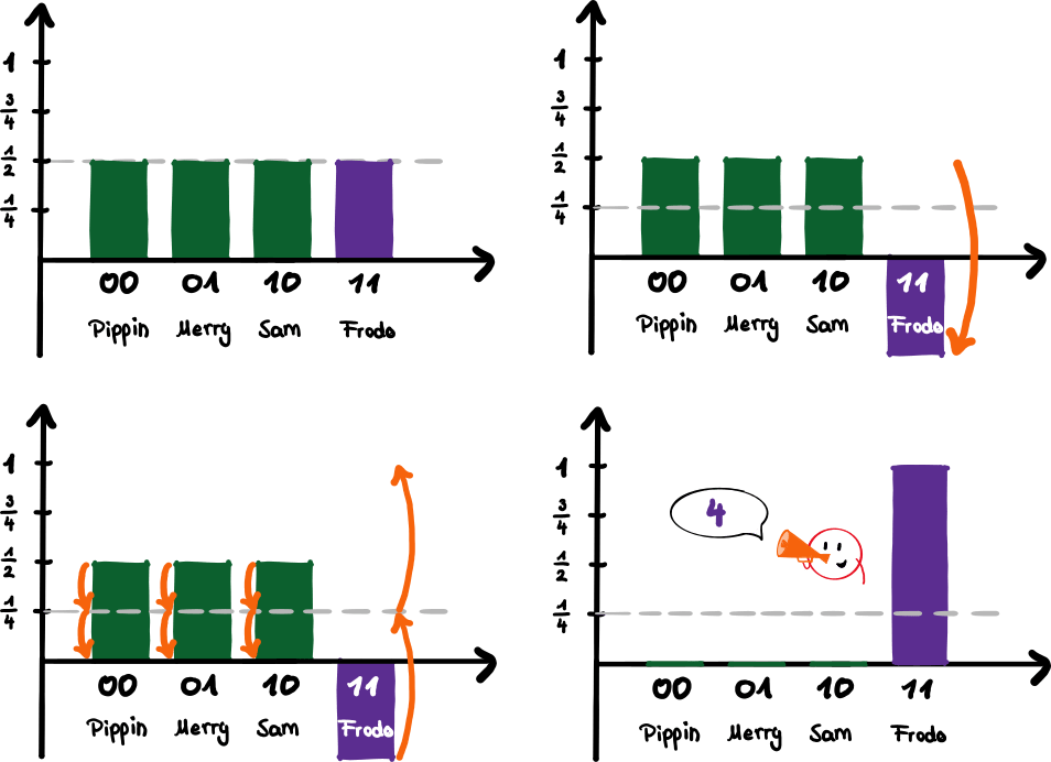
Initial situation: Groping in the dark

We are at the beginning and have no idea where Frodo is (picture top left). This means that the probability of finding Frodo by chance is 25%. The probability for the other hobbits is just as high. A word about the bar chart in the picture: The y-axis (the one pointing upwards) does not indicate the probability of finding a name on the list. Instead, it shows the quantum mechanical “pre-factor” of the four states 00, 01, 10, 11. When this number is squared we get the probability of measuring that state $\left(\frac{1}{2} \cdot \frac{1}{2} = \frac{1}{4} = 25\%\right)$ . But we are not doing that yet!

Step 1: Mirroring Frodo

With the help of a quantum operation, we can reverse the sign of the element we are looking for (picture top right; the y-axis thus definitely shows no probabilities, since the value is now negative and negative probabilities do not exist). But with this we have not yet found Frodo, since the probability of measuring Frodo is still 25% $\left( \frac{-1}{2} \cdot \frac{-1}{2} = \frac{1}{4} = 25\%\right)$ . With the help of quantum physics, however, we can “feel” into the list – the two qubits already sense Frodo. But we cannot do anything with this information.

Step 2: Mirroring all Hobbits

Now we mirror all four columns (picture bottom left). However, not on the x-axis (pointing to the right), but on the mean value of the four columns (the grey dashed line). Since Frodo is negative, the mean of the four amplitudes is $\left( \frac{1}{2} + \frac{1}{2} + \frac{1}{2} - \frac{1}{2}\right) / 4 = 1 / 4$ . The reflection is illustrated by the orange arrows.

Frodo reveals himself

The mirroring has led us to our goal (picture bottom right)! The amplitude of Pippin, Merry and Sam is now 0, that of Frodo is 1. If we now read out the two qubits, we will find Frodo with 100% probability!

However, it is not always as easy as in this example with only four entries. So now a few more notes for those who want to know more:

“Why do you call that one step, wasn’t that several steps?” Yes, that is a question of definition. We did two operations above (the two reflections) and one measurement (the last step). In fact, to perform the two reflections on a real quantum computer, several quantum gates are needed. However, all this can be interpreted as one complex quantum operation. And it is precisely this that is repeated again and again in the case of a longer list. In any case, we perform only one measurement at the very end.
“Can this always be done in one step?” Only for the case of four list entries can the Grover algorithm find the element in one step. In all other cases, steps one and two must be repeated several times.
“Wait a minute, why one step at all? You said the Grover algorithm takes $\sqrt{N}$ steps to find the element, but $\sqrt{4} = 2$ and not 1!” In fact, the Grover algorithm does not require exactly $\sqrt{N}$ steps, but the number of steps scales with $\sqrt{N}$ . The formula $\frac{\sqrt{N}}{2}$ also scales with $\sqrt{N}$ and also the formula $1,000,000 \sqrt{N}$ scales with $\sqrt{N}$ . The question is how much the number of steps increases as the list gets longer. The exact formula for the Grover algorithm is a little more complicated but the factor $\sqrt{N}$ appears in it. For three qubits, that is $2^3 = 2\cdot 2 \cdot 2 = 8$ list entries, 1-2 steps are needed, for five qubits ( $2^5 = 32$ entries) just four!
“How do you do these reflections?” They look quite easy in a diagram but we need to get the qubits to behave in exactly the same way. We do this with the help of quantum gates. In practical terms, this means that we shoot electromagnetic pulses at the qubits, for example, to make their arrows spin in a very specific way.
“Do all quantum algorithms have anything in common?” The basic concept on which all quantum algorithms are based is interference (more on that here), i.e. the superposition of matter waves: The “bad” list entries interfere destructively so that their amplitudes eventually become (almost) zero. The “good” list entry interferes constructively so that its amplitude becomes (almost) one. This can be seen well in the second reflection: it simply cancels the bad entries and amplifies the good one.

What can quantum computers do better than normal computers?

Roughly speaking, quantum computers are always superior to normal ones if you could find the solution by mere guesswork and trial and error. Finding elements in a list, decomposing numbers into their factors, cracking passwords, optimising things. The German railway company Deutsche Bahn, for example, hopes to optimise its route networks with quantum computers in the future (about time).

There is one thing a quantum computer can do that a classical computer cannot: Generate random numbers. You might be surprised by this because even on the internet there are random number generators. That doesn’t seem to be a problem, does it? Not quite, because it is actually a super difficult task to generate perfectly random numbers.

In everyday life, it’s not that difficult to generate random numbers: take a coin or a dice, for example. But if you look closely, the result is not random: if I know all the external parameters of the dice throw, I can calculate the result. All I need is the force with which I throw the dice, the material of the dice and the table, the position of the dice in my hand, the angle at which I throw it, the wind speed, the temperature, the constellation of stars, … Um, yes. You see, so many parameters go into a simple throw of the dice which we don’t know precisely enough in practice, so it’s impossible to predict the outcome exactly. That’s why we can say with a clear conscience: the result is random.

But how does a computer do that? A computer does not have a dice. Computers are designed to carry out calculations: Take A and do B with it, and then tell me the result C. A computer is overwhelmed with the task: do what you want, but don’t tell me, only tell me the result. That’s why random numbers from computers are only pseudo-random. The numbers look random, but in fact there is a complicated calculation hidden that spits out predictable numbers.

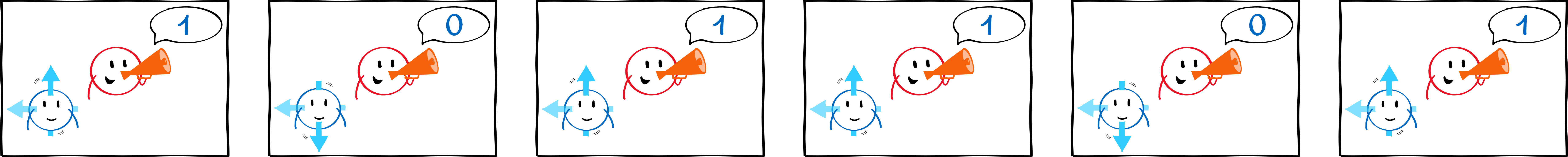
But a quantum computer is different. In quantum physics, we can only predict the state of a qubit with a certain probability. A qubit in a superposition of states 0 and 1 returns state 0 with 50% probability and state 1 with 50% probability. Tada: our 100% random quantum coin! With nothing in the world can we predict the outcome of this coin toss.

What can normal computers do better than quantum computers?

Roughly speaking: everything else (i.e. except finding elements in a list, decomposing numbers into their factors, cracking passwords, optimising things,…). If we don’t know a quantum algorithm that solves a problem with quantum power, then a quantum computer is useless. As explained above, quantum computers can basically do everything that classical computers can do – only worse.

However, there is one thing that quantum computers actually cannot do: Copying. One of the most important results of quantum physics is the no-cloning theorem. It states that it is impossible to copy any qubit. To copy the state of a qubit, I first have to know what that state actually is. With classical bits, this is quite simple: I look at a bit (Does the switch point up or down?) and flip the switch of another bit to exactly the same position – done. This “looking at” is not so simple with qubits, however, because just looking at something usually affects the qubit. The simple assignment a = b is not possible on a quantum computer.

Snitch in message transmission — A normally encrypted message is intercepted by a snitch who retransmits a copy.

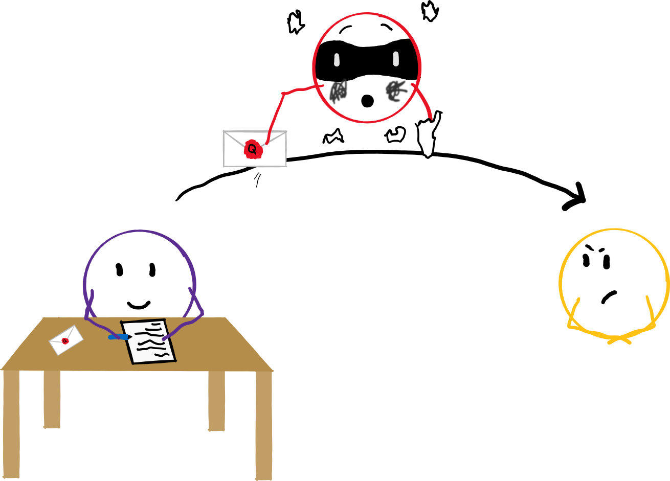
This sounds rather obstructive if you want to build a computer. But in fact, this very property is the key to quantum cryptography! One of the goals of quantum cryptography is to make message transmission uninterceptable. When snitch wants to intercept normal messages, they intercept them, read the message and send it (or a copy of it) on. The recipient can never know for sure whether a snitch has intercepted the message. Quantum messages are naturally protected from such attacks because they cannot be read undamaged, nor can they be copied and sent on.

quantum transmission — A quantum-encrypted message cannot be intercepted without breaking it. The recipient notices that the message has been intercepted.

How many qubits does a quantum computer have?

The record for the highest number of qubits is currently held by Google with 72. IBM is close behind with 65 – the two regularly beat each other. The really relevant question, however, is: how many qubits do we need to do useful things? Counter question: What is useful?

The prime example of quantum computing is cracking encryption. The most important method is RSA encryption, which is used for credit cards, emails, passports and for much more. It is based, simply put, on prime factorisation: While it is still easy to decompose small numbers like 15 into factors of 3 and 5, an enormous amount of computation is required for a number with several hundred digits. RSA-2048 uses 2048 bits for encryption, resulting in a number with 617 digits. To decompose such a large number into its prime factors would take 300 trillion years on a classical computer – so it is not too much to say that this is considered impossible. If, on the other hand, you had a quantum computer with just under 4000 perfect qubits, you could crack the code in 10 seconds.

That is why another field of research has already developed: Post-quantum cryptography. Because as soon as we have a 4000 qubit quantum computer, our credit cards are unprotected. It’s the circle of life: we solve problems and directly create new ones to solve.

Don’t quantum computers already exist?

When you get right down to it: Yes. However, they are not yet the overpowering, code-breaking machines that everyone dreams of. Today’s quantum computers can be divided into three categories:

Adiabatic quantum computers

When you open the website of the Canadian company D-Wave Systems, the first words you read are “The first and only quantum computer built for business”. Clear announcement. Back in 2011, the company claimed to have developed the first commercial quantum computer. They sold their device D-Wave One for US$10 million. However, the devil is in the detail, because the device is not a quantum computer in the sense I am using it here. It does not work with quantum gates and cannot execute the usual quantum algorithms. So although the latest D-Wave Advantage device has 5760 qubits, we don’t need to fear for our security yet – for Shor’s algorithm you need a “real” quantum computer. The D-Wave devices are instead so-called adiabatic quantum computers. The principle of operation is as follows:

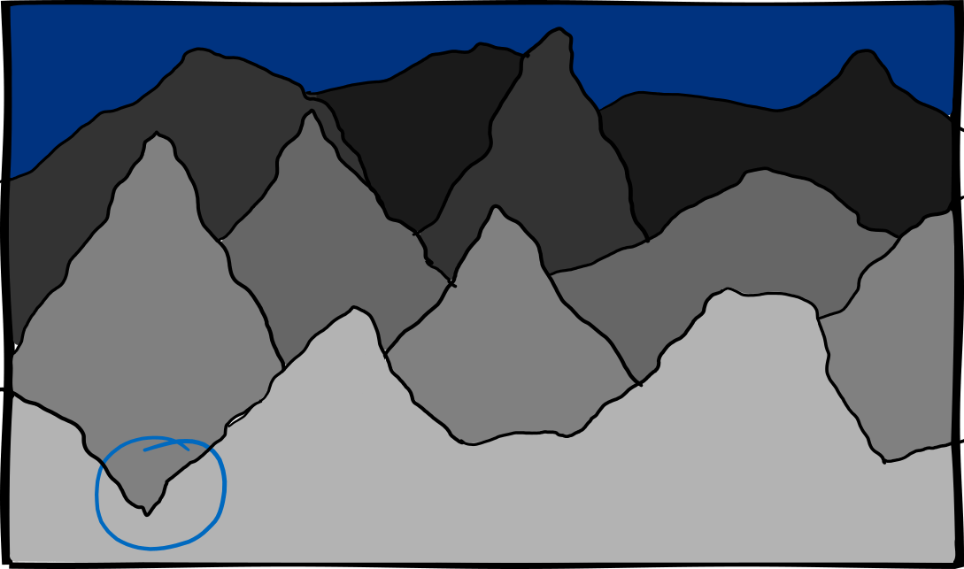
Landscape — The optimisation as a landscape. The goal is to find the lowest point (blue circle).

With the help of adiabatic quantum computers, optimisation problems can be solved. That is, one tries to find the minimum or maximum of a process. You can imagine an optimisation as a landscape, and the goal is to find the lowest point. Let’s say we have the model of the landscape in a box in front of us. An adiabatic quantum computer then looks at each point simultaneously by (figuratively speaking) sprinkling flour on the landscape. We then carefully shake the box until all the flour collects at the lowest point. It is important to shake the box slowly and gently because “adiabatic” is a physical term for “super slow”: if we shake too hard, the flour can bounce over small bumps and does not land at the lowest point. Quantum flour also has the advantage that it can jump through mountains when it notices that it is going further down on the other side. This is what we call tunneling. That’s why adiabatic quantum computers are well suited to solving optimisation problems like this.

Quantum computer of the NISQ era

Chinese company SpinQ Technology says on its website “Gemini is the world’s first commercially available desktop quantum computer.” Sounds great, and only cost US$50,000. The next generation, announced for the end of the year, is said to cost as little as $5000. However, if you read a little further you find the addition of “It provides a comprehensive solution for teaching and demonstrating quantum computing.” This is because the SpinQ Gemini consists of only two qubits. You can’t really crack codes with it (but you can find Frodo!)

As described above, we need 4000 qubits to crack the best encryption. But even a few dozen perfect qubits could solve relevant problems (it doesn’t always have to be the breaking of the global high-security encryption system). The only problem is that today’s qubits are anything but perfect. They are unstable and give a wrong result with a certain probability. The main reason for this is decoherence: the decay of quantum information over time (see “Why is it so hard to build a quantum computer?” in the last article).

We are currently in a grey area: the so-called NISQ era, for Noisy Intermediate Scale Quantum. This means that the number of qubits is already large enough (intermediate scale) to solve complex problems, but the results are distorted by noise (noisy). The holy grail of quantum computing is a device with built-in error correction. The idea is to correct the errors of the noisy qubits with the help of additional qubits. How many qubits are needed for error correction is still unclear but a ratio of 1:10 is suspected. Since one of the biggest problems at present is to scale up the number of qubits, error-tolerant quantum computers are not yet feasible.

If we include error correction, the number of qubits increases significantly to crack RSA. Recent calculations show that it takes 20 million qubits to crack the encryption in just eight hours. That’s quite a bit more than 4000, and a lot more than the 70 we currently have. It will probably be decades before we get there.

Cloud-based quantum computers

IBM has been allowing the general public access to its quantum computers since 2016 – via the internet. The project was launched under the name IBM Quantum Experience and was recently split into two components: IBM Quantum Composer (for drag-and-drop creation of quantum circuits) and IBM Quantum Lab (for programming using a programming language adapted for quantum computers). IBM allows users to access its quantum processors with between one and 65 qubits. The company calls this access via the Internet the IBM Cloud.

So instead of having a quantum computer at home, we can access cloud-based quantum computers remotely. The idea is the same as with cloud gaming: games are no longer installed locally on your own computer but on an external server. The gamer’s keyboard and mouse input is sent to the server, and the server sends back image and sound, all via the internet.

The advantage of this is that the sensitive qubits are safely packed in a cryostat or vacuum somewhere far away in a quantum server room. There are also platforms that don’t need these extreme conditions (see “What are qubits made of?” in Part One), but they are still usually better for performance. All the big-name representatives of quantum computing now offer cloud access: IBM, Google, D-Wave, Amazon and many more.

When will there be home quantum computers?

I’ll be bold and say: Probably never. As explained in “What can quantum computers do better than normal ones?”, quantum computers mainly shine in areas that you don’t really need as a normal user (unless you are a professional hacker or a freelance spy). IF quantum computers ever do play a role at home, my guess is that it will be via the cloud, as this development has already begun. Especially since researchers are simply not working on developing home quantum computers.

In fact, it’s even remotely about developing quantum computers for industrial production. We are still in the research phase: is it even possible to develop a quantum computer that can solve significant problems that a normal computer could not (in reasonable time)? NISQ-era devices are products of this research, but they are not yet the final result. Most researchers are confident and it only sounds like a matter of time. But until we actually hold the “holy grail” in our hands, we cannot be sure that we will really find it.

Do you like what you read? Then subscribe to my blog and never miss a new post again! Or if you like, you could buy me a coffee here!

References
Grover Algorithmus
Breaking RSA Encryption – an Update on the State-of-the-Art
How to factor 2048 bit RSA integers in 8 hours using 20 million noisy qubits
IBM Quantum Experience
D-Wave Leap
Google Quantum Computing Playground (formerly http://quantumplayground.net/, accessed on 04/2022)
Amazon Braket Quantencomputer
SpinQ Gemini: a desktop quantum computer for education and research
SpinQ Website

FAQ: Quantum Computer – From classical to quantum computer